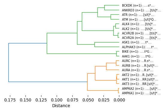
Hierarchical clustering

Setup

KL divergence

kl_divergence

 kl_divergence (p1, p2, mean=True)

*KL divergence D_KL(p1 || p2) over positions.

p1 and p2 are arrays (df or np) with index as aa and column as position. Returns average divergence across positions if mean=True, else per-position.*

	Type	Default	Details
p1			target pssm p (array-like, shape: (AA, positions))
p2			pred pssm q (array-like, same shape as p1)
mean	bool	True

The Kullback–Leibler (KL) divergence between two probability distributions ( P ) and ( Q ) is defined as:

\[ \mathrm{KL}(P \| Q) = \sum_{x \in \mathcal{X}} P(x) \log \left( \frac{P(x)}{Q(x)} \right) \]

This measures the information lost when ( Q ) is used to approximate ( P ). It is not symmetric, i.e.,

\[ \mathrm{KL}(P \| Q) \ne \mathrm{KL}(Q \| P) \]

and it is non-negative, meaning:

\[ \mathrm{KL}(P \| Q) \ge 0 \]

with equality if and only if ( P = Q ) almost everywhere.

In practical computation, to avoid numerical instability when ( P(x) = 0 ) or ( Q(x) = 0 ), we often add a small constant ( ):

\[ \mathrm{KL}_\varepsilon(P \| Q) = \sum_{x \in \mathcal{X}} P(x) \log \left( \frac{P(x) + \varepsilon}{Q(x) + \varepsilon} \right) \]

pssms = Data.get_pspa_all_scale()

pssm_df.shape

(23, 10)

# one example
pssm_df = recover_pssm(pssms.iloc[1])
pssm_df2 = recover_pssm(pssms.iloc[0])

kl_divergence(pssm_df,pssm_df2,mean=True)

0.3724275257321628

source

kl_divergence_flat

 kl_divergence_flat (p1_flat, p2_flat)

p1 and p2 are two flattened pd.Series with index as aa and column as position

	Details
p1_flat	pd.Series of target flattened pssm p
p2_flat	pd.Series of pred flattened pssm q

kl_divergence_flat(pssms.iloc[1],pssms.iloc[0])

CPU times: user 2.83 ms, sys: 322 μs, total: 3.15 ms
Wall time: 3.21 ms

0.37242752573216287

JS divergence

source

js_divergence

 js_divergence (p1, p2, mean=True)

p1 and p2 are two arrays (df or np) with index as aa and column as position

	Type	Default	Details
p1			pssm
p2			pssm
mean	bool	True

The Jensen-Shannon divergence between two probability distributions $ P $ and $ Q $ is defined as:

\[ \mathrm{JS}(P \| Q) = \frac{1}{2} \, \mathrm{KL}(P \| M) + \frac{1}{2} \, \mathrm{KL}(Q \| M) \]

where $ M = (P + Q) $ is the average (mixture) distribution, and $ $ denotes the Kullback–Leibler divergence:

\[ \mathrm{KL}(P \| Q) = \sum_{x \in \mathcal{X}} P(x) \log \left( \frac{P(x)}{Q(x)} \right) \]

Therefore,

\[ \mathrm{JS}_\varepsilon(P \| Q) = \frac{1}{2} \sum_{x \in \mathcal{X}} P(x) \log \left( \frac{P(x) + \varepsilon}{M(x) + \varepsilon} \right) + \frac{1}{2} \sum_{x \in \mathcal{X}} Q(x) \log \left( \frac{Q(x) + \varepsilon}{M(x) + \varepsilon} \right) \]

js_divergence(pssm_df,pssm_df2)

0.08286124552178498

js_divergence(pssm_df,pssm_df)

0.0

# don't use it for flattend version, as it won't divide the total position
js_divergence(pssms.iloc[1],pssms.iloc[0])

0.8286124552178498

source

js_divergence_flat

 js_divergence_flat (p1_flat, p2_flat)

p1 and p2 are two flattened pd.Series with index as aa and column as position

	Details
p1_flat	pd.Series of flattened pssm
p2_flat	pd.Series of flattened pssm

js_divergence_flat(pssms.iloc[1],pssms.iloc[0])

CPU times: user 1.23 ms, sys: 0 ns, total: 1.23 ms
Wall time: 1.2 ms

0.08286124552178498

source

js_divergence_flat2

 js_divergence_flat2 (p1_flat, p2_flat, mean=True)

p1 and p2 are two flattened pd.Series with index as aa and column as position

	Type	Default	Details
p1_flat			pd.Series of flattened pssm
p2_flat			pd.Series of flattened pssm
mean	bool	True

js_divergence_flat2(pssms.iloc[1],pssms.iloc[0])

CPU times: user 11.2 ms, sys: 0 ns, total: 11.2 ms
Wall time: 10.1 ms

0.08286124552178498

js_divergence_flat2(pssms.iloc[1],pssms.iloc[0],mean=False)

CPU times: user 10 ms, sys: 0 ns, total: 10 ms
Wall time: 9.18 ms

array([0.06553878, 0.02571207, 0.05479896, 0.10319209, 0.08337669,
       0.10549031, 0.34404931, 0.00729907, 0.02094918, 0.018206  ])

This version is slower as it recover flat pssm to 2d pssm first, but it can return positional js.

source

get_1d_distance

 get_1d_distance (df, func_flat)

Compute 1D distance for each row in a dataframe given a distance function

# return 1d distance
get_1d_distance(pssms.head(),js_divergence_flat)

100%|█████████████████████████████████████████████████████████████████████████████████████████████| 5/5 [00:00<00:00, 301.61it/s]

array([0.08286126, 0.08577979, 0.08798377, 0.0850101 , 0.00215833,
       0.07937985, 0.07066438, 0.08348297, 0.07361696, 0.00425251])

source

get_1d_js

 get_1d_js (df)

Compute 1D distance using JS divergence.

distance = get_1d_js(pssms.head(20))

100%|████████████████████████████████████████████████████████████████████████████████████████████| 20/20 [00:00<00:00, 69.75it/s]

Parallel computing to accelerate when flattened pssms are too many in a df:

source

get_1d_distance_parallel

 get_1d_distance_parallel (df, func_flat, max_workers=4, chunksize=100)

Parallel compute 1D distance for each row in a dataframe given a distance function

get_1d_distance_parallel(pssms.head(),js_divergence_flat)

source

get_1d_js_parallel

 get_1d_js_parallel (df, func_flat=<function js_divergence_flat>,
                     max_workers=4, chunksize=100)

Compute 1D distance matrix using JS divergence.

get_1d_js_parallel(pssms.head())

source

get_Z

 get_Z (pssms, func_flat=<function js_divergence_flat>, parallel=True)

Get linkage matrix Z from pssms dataframe

Z = get_Z(pssms.head(10),parallel=False)

100%|███████████████████████████████████████████████████████████████████████████████████████████| 10/10 [00:00<00:00, 144.66it/s]

Z[:5]

array([[1.00000000e+00, 2.00000000e+00, 2.15832816e-03, 2.00000000e+00],
       [3.00000000e+00, 4.00000000e+00, 4.25250792e-03, 2.00000000e+00],
       [5.00000000e+00, 1.10000000e+01, 4.65131778e-03, 3.00000000e+00],
       [6.00000000e+00, 7.00000000e+00, 5.89060764e-03, 2.00000000e+00],
       [1.00000000e+01, 1.30000000e+01, 9.31413380e-03, 4.00000000e+00]])

source

plot_dendrogram

 plot_dendrogram (Z, color_thr=0.07, dense=7, line_width=1, **kwargs)

	Type	Default	Details
Z
color_thr	float	0.07
dense	int	7	the higher the more dense for each row
line_width	int	1
kwargs	VAR_KEYWORD

set_sns(100)

plot_dendrogram(Z,dense=7,line_width=1)

plot_dendrogram(Z,dense=4)

source

pssm_to_seq

 pssm_to_seq (pssm_df, thr=0.2, clean_center=True)

Represent PSSM in string sequence of amino acids

	Type	Default	Details
pssm_df
thr	float	0.2	threshold of probability to show in sequence
clean_center	bool	True	if true, zero out non-last three values in position 0 (keep only s,t,y values at center)

pssm_to_seq(pssm_df,thr=0.1)

'...[E/D].[t/s]*[s/t]...'

source

get_pssm_seq_labels

 get_pssm_seq_labels (pssms, count_map=None, thr=0.3)

Use index of pssms and the pssm to seq to represent pssm.

	Type	Default	Details
pssms
count_map	NoneType	None	df index as key, counts as value
thr	float	0.3	threshold of probability to show in sequence

get_pssm_seq_labels(pssms.head(10))

['AAK1: .....t*G...',
 'ACVR2A: .....[t/s]*....',
 'ACVR2B: .....[t/s]*....',
 'AKT1: ..RR.[s/t]*....',
 'AKT2: ..R..[s/t]*....',
 'AKT3: ..RR.[s/t]*....',
 'ALK2: .....[t/s]*....',
 'ALK4: .....[t/s]*....',
 'ALPHAK3: .....t*....',
 'AMPKA1: .....[s/t]*....']

import random

# get a dict of index and counts

count_dict = {idx:random.randint(1,100) for idx in pssms.head(10).index}

labels= get_pssm_seq_labels(pssms.head(10),count_dict)
labels

['AAK1 (n=64): .....t*G...',
 'ACVR2A (n=56): .....[t/s]*....',
 'ACVR2B (n=30): .....[t/s]*....',
 'AKT1 (n=37): ..RR.[s/t]*....',
 'AKT2 (n=94): ..R..[s/t]*....',
 'AKT3 (n=68): ..RR.[s/t]*....',
 'ALK2 (n=86): .....[t/s]*....',
 'ALK4 (n=79): .....[t/s]*....',
 'ALPHAK3 (n=64): .....t*....',
 'AMPKA1 (n=88): .....[s/t]*....']

plot_dendrogram(Z,dense=4,labels=labels)

Full pipeline

# get distance matrix
pssms=pssms.head(100)

Z = get_Z(pssms)

# optional, get counts for each index
# count_dict = pssms.index.value_counts()

# get pssm to seq labels with counts
# labels= get_pssm_seq_labels(pssms,count_dict)

# or get pssm to seq labels only
labels= get_pssm_seq_labels(pssms)

# plot dendrogram
plot_dendrogram(Z,dense=8,labels=labels,truncate_mode='lastp', p=40) # only show 40

# save
# save_pdf('dendrogram.pdf')

Setup

KL divergence

kl_divergence

kl_divergence_flat

JS divergence

js_divergence

js_divergence_flat

js_divergence_flat2

get_1d_distance

get_1d_js

get_1d_distance_parallel

get_1d_js_parallel

get_Z

plot_dendrogram

pssm_to_seq

get_pssm_seq_labels

Full pipeline

End