pssm.lo

calculation of log-odds PSSM and visualization

Overview

Log-Odds PSSM Calculation

To compute a log-odds Position-Specific Scoring Matrix (PSSM) by comparing observed amino acid frequencies against a background model:

pssm_LO = get_pssm_LO(
    pssm_df=pssm_df,    # DataFrame of amino acid frequencies (rows=aa, cols=positions)
    site_type='STY',    # background model: 'S', 'T', 'Y', 'ST', or 'STY'
)

To compute a log-odds PSSM from a flattened (1D) frequency representation:

pssm_LO = get_pssm_LO_flat(
    flat_pssm=flat_pssm,  # flattened PSSM as pd.Series
    site_type='STY',      # background model: 'S', 'T', 'Y', 'ST', or 'STY'
)

Log-Odds Visualization

To visualize a log-odds PSSM as a sequence logo where letter heights reflect enrichment/depletion:

plot_logo_LO(
    pssm_LO=pssm_LO,        # log-odds PSSM DataFrame
    title='Motif',          # plot title
    acceptor=None,          # force display of central residue: 'S', 'T', or 'Y'
    scale_zero=True,        # rescale position 0 to match max stack height
    scale_pos_neg=True,     # normalize positive/negative stacks for visibility
    ax=None,                # matplotlib Axes (creates new if None)
    figsize=(10, 1),        # figure dimensions (width, height)
)

To display both a sequence logo and a heatmap of log-odds values in a combined figure:

plot_logo_heatmap_LO(
    pssm_LO=pssm_LO,        # log-odds PSSM DataFrame
    title='Motif',          # plot title
    acceptor=None,          # force display of central residue: 'S', 'T', or 'Y'
    figsize=(17, 10),       # figure dimensions (width, height)
    include_zero=False,     # include position 0 in heatmap
    scale_pos_neg=True,     # normalize color scale for positive/negative values
)

Setup

from katlas.data import *

data = Data.get_ks_dataset()
data_k = data[data.kinase_uniprot=='P49841'] # CDK1
pssm_df=get_prob(data_k, col='site_seq')

Calculate

get_pssm_LO


def get_pssm_LO(
    pssm_df, site_type, # S, T, Y, ST, or STY
):

Get log odds PSSM: log2 (freq pssm/background pssm).

Let \(P_i(x)\) be the frequency of amino acid \(x\) at position \(i\) in the input PSSM, and let \(B_i(x)\) be the background frequency of amino acid \(x\) at the same position, derived from a background model corresponding to the specified site type (S, T, Y, or STY).

The log-odds score at each position \(i\) for amino acid \(x\) is computed as:

\[ \mathrm{LO}_i(x) = \log_2 \left( \frac{P_i(x) + \varepsilon}{B_i(x) + \varepsilon} \right) \]

where \(\varepsilon = 10^{-8}\) is a small constant added for numerical stability and to avoid division by zero.

This results in a matrix where:

Positive values indicate enrichment over background,
Negative values indicate depletion relative to background,
Zero indicates no difference from the expected background.

pssm_LO = get_pssm_LO(pssm_df,'STY')
pssm_LO.head()

Position	-20	-19	-18	-17	-16	-15	-14	-13	-12	-11	-10	-9	-8	-7	-6	-5	-4	-3	-2	-1	0	1	2	3	4	5	6	7	8	9	10	11	12	13	14	15	16	17	18	19	20
aa
P	0.059908	0.281140	-0.026749	0.355318	0.346468	0.178779	0.463147	0.308758	0.239997	0.179283	0.608034	0.192985	0.329370	0.721201	0.715760	0.588674	0.320993	1.112040	0.973481	1.055403	0.0	1.539081	1.109428	0.434700	-0.301588	1.379883	0.314032	0.243357	-0.060158	0.644231	0.061865	0.161917	0.308782	0.140834	0.521194	0.373708	0.158627	0.462854	0.138734	0.658643	0.216764
G	0.355425	0.331928	0.015762	-0.090070	0.155057	-0.318908	0.274539	0.486357	-0.081333	-0.044640	-0.023817	0.297183	-0.167014	-0.096944	-0.092276	-0.064319	-0.075365	0.473975	0.243292	0.358158	0.0	0.235499	-0.025131	0.284594	-0.457652	-0.327199	-0.123033	0.303309	0.315783	-0.190655	-0.067465	0.298568	0.361469	0.170286	0.215167	0.258789	-0.054255	-0.185829	0.200256	0.388134	-0.066157
A	0.445724	0.399204	0.032468	0.105841	0.037853	0.527832	0.039466	-0.201953	0.117073	0.243623	0.053728	-0.015571	0.335906	0.169137	-0.130969	-0.098714	-0.444541	0.119458	0.286568	0.060413	0.0	-0.584316	0.490663	-0.075931	-0.078570	0.109301	0.496097	0.191241	-0.008452	-0.306504	0.241955	-0.675462	-0.013856	0.172464	-0.080489	-0.019176	0.360468	0.315254	0.109869	-0.375457	0.164260
C	0.537945	-0.956246	-0.269417	-0.055141	-0.547438	-0.718577	-0.987818	0.075745	0.419542	-0.634510	-0.603081	-0.233384	0.494481	0.142392	0.851304	0.003453	-0.677106	-0.935493	0.789298	0.156753	0.0	-0.937435	0.945576	0.925658	-1.573420	-1.149739	0.860460	-0.169595	-0.143715	0.200914	-0.385030	0.235879	0.725572	-0.115854	0.491228	-0.070391	-0.647993	-0.426118	1.057556	-1.543537	-0.898042
S	0.482063	0.128128	0.452159	-0.214803	0.139830	0.049341	0.317830	-0.214082	0.175540	-0.036560	0.017835	0.187378	0.362312	-0.239848	0.014115	0.612648	-0.070659	-0.737274	0.126846	0.744032	0.0	-0.314505	0.076891	0.803635	0.224781	-0.198496	0.474760	0.303879	0.367185	-0.142147	0.492529	0.309106	-0.086104	-0.016800	-0.160346	-0.145271	-0.167390	-0.262078	0.101268	0.189145	0.426381

get_pssm_LO_flat


def get_pssm_LO_flat(
    flat_pssm, site_type, # S, T, Y, ST, or STY
):

flat_pssm=pd.Series(flatten_pssm(pssm_df))

pssm_LO = get_pssm_LO_flat(flat_pssm,'STY')
pssm_LO

Position	-20	-19	-18	-17	-16	-15	-14	-13	-12	-11	-10	-9	-8	-7	-6	-5	-4	-3	-2	-1	0	1	2	3	4	5	6	7	8	9	10	11	12	13	14	15	16	17	18	19	20
aa
P	0.059908	0.281140	-0.026749	0.355318	0.346468	0.178779	0.463147	0.308758	0.239997	0.179283	0.608034	0.192985	0.329370	0.721201	0.715760	0.588674	0.320993	1.112040	0.973481	1.055403	0.000000	1.539081	1.109428	0.434700	-0.301588	1.379883	0.314032	0.243357	-0.060158	0.644231	0.061865	0.161917	0.308782	0.140834	0.521194	0.373708	0.158627	0.462854	0.138734	0.658643	0.216764
G	0.355425	0.331928	0.015762	-0.090070	0.155057	-0.318908	0.274539	0.486357	-0.081333	-0.044640	-0.023817	0.297183	-0.167014	-0.096944	-0.092276	-0.064319	-0.075365	0.473975	0.243292	0.358158	0.000000	0.235499	-0.025131	0.284594	-0.457652	-0.327199	-0.123033	0.303309	0.315783	-0.190655	-0.067465	0.298568	0.361469	0.170286	0.215167	0.258789	-0.054255	-0.185829	0.200256	0.388134	-0.066157
...	...	...	...	...	...	...	...	...	...	...	...	...	...	...	...	...	...	...	...	...	...	...	...	...	...	...	...	...	...	...	...	...	...	...	...	...	...	...	...	...	...
t	0.338037	-0.508472	0.536544	0.409825	0.546294	0.066828	0.190809	-0.298146	0.023876	0.295761	0.995227	1.015112	0.246666	-0.332277	0.195250	0.680780	1.210743	0.166721	0.546415	-0.157283	0.329833	-0.420698	-0.286888	0.507349	1.536109	0.349480	0.508819	1.032751	0.944610	0.697806	1.386345	0.723589	0.986439	-0.036165	0.368048	-0.516571	-0.021008	0.119857	0.161114	-0.047991	-0.097686
y	-1.109821	0.265760	-0.184739	0.075387	0.307806	0.041911	-0.180464	-1.440588	-0.516052	0.508038	-0.011805	0.496492	-0.749242	0.261563	0.139186	0.233321	-1.138437	-1.195610	-1.747661	-1.166771	-2.655631	-0.065791	-1.535247	-0.045814	0.191191	-1.732180	-1.613038	-0.465142	-0.886647	-0.336320	-0.712011	0.069406	-0.161659	-0.829713	0.474154	-0.851437	-0.438485	-0.267581	0.642920	-0.356680	0.230591

23 rows × 41 columns

Plot

plot_logo_LO


def plot_logo_LO(
    pssm_LO, title:str='Motif', acceptor:NoneType=None, scale_zero:bool=True, scale_pos_neg:bool=True,
    ax:NoneType=None, figsize:tuple=(10, 1)
):

Plot logo of log-odds given a frequency PSSM.

To ensure the phosphorylated residue is visible at the center of a log-odds motif (position 0), two mechanisms are used:

Acceptor override: If the center column is entirely zero (e.g., masked), the user can specify an acceptor ('S', 'T', 'Y', or 'STY'). The function then assigns a small nonzero value (e.g., 0.1) to the corresponding phospho-residue row (pS, pT, pY) at position 0. This ensures the central letter appears in the logo plot, even when real log-odds values are absent.
Stack height rescaling: To maintain visual consistency with surrounding columns, position 0 is rescaled so that its total positive and negative stack heights match the most extreme values observed elsewhere.

Together, these adjustments ensure that: - The phospho-acceptor appears explicitly at the center, - The visual scale remains consistent with neighboring positions, - The resulting logo can faithfully reflect both biological relevance and statistical signal.

pssm_LO = get_pssm_LO(pssm_df,'STY')
plot_logo_LO(pssm_LO,scale_zero=False,scale_pos_neg=False)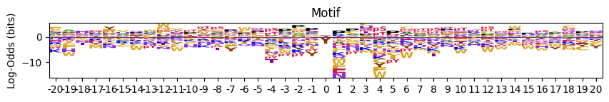

# with zero position scaled to the max
plot_logo_LO(pssm_LO,scale_zero=True,scale_pos_neg=False)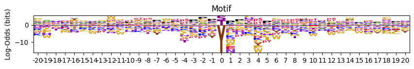

# scaled positive and negative values for better visualization
plot_logo_LO(pssm_LO,scale_zero=True,scale_pos_neg=True)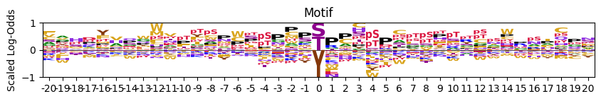

# # for those specific site type (S,T or Y), show acceptor in the middle instead of empty
# pssm_LO = get_pssm_LO(pssm_y,'Y')
# plot_logo_LO(pssm_LO,acceptor='Y')

plt.close('all')

plot_logo_heatmap_LO


def plot_logo_heatmap_LO(
    pssm_LO, # pssm of log-odds
    title:str='Motif', acceptor:NoneType=None, figsize:tuple=(17, 10), include_zero:bool=False,
    scale_pos_neg:bool=True
):

Plot logo and heatmap of enrichment bits vertically

# plot_logo_heatmap_LO(pssm_LO,acceptor='Y')

pssm_LO = get_pssm_LO(pssm_df,'STY')
plot_logo_heatmap_LO(pssm_LO,scale_pos_neg=False) # normal color scale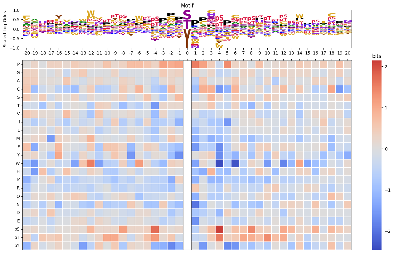

plt.close('all')