kplot

kplot is a Python plotting toolkit for exploratory data analysis. It provides reusable helpers for styling figures, scatter and embedding plots, categorical summaries, heatmaps, hierarchical clustering, and related ranking workflows.

Installation

pip install python-kplot

Quick start

The examples below follow the notebooks under nbs/ in order. Each function example lives in its own cell and starts with a short comment derived from the function docstring.

01 utils

from kplot.utils import set_sns, save_svg, save_pdf, save_show, get_color_dict, get_plt_color, get_hue_big, add_stats

import seaborn as sns
from matplotlib import pyplot as plt

# Set up the objects used by the examples below.
df = sns.load_dataset('tips')
df.shape

(244, 7)

# Set seaborn defaults for notebook display and saved figures.
set_sns(dpi=50)

# Save the current matplotlib figure as SVG with editable text.
plt.figure()
plt.plot([0, 1], [0, 1])
# save_svg(Path('nbs') / '_tmp_utils.svg')

# Save the current matplotlib figure as PDF with TrueType fonts.
plt.figure()
plt.plot([0, 1], [1, 0])
# save_pdf(Path('nbs') / '_tmp_utils.pdf')

# Show the current figure or save it, then close open figures.
plt.figure()
plt.plot([0, 1], [0.5, 0.5])
# save_show(path=Path('nbs') / '_tmp_utils_show.png')

# Assign colors to labels while tolerating duplicate category names.
get_color_dict(['A', 'B', 'C'], palette='Set2')

{'A': (0.4, 0.7607843137254902, 0.6470588235294118),
 'B': (0.9882352941176471, 0.5529411764705883, 0.3843137254901961),
 'C': (0.5529411764705883, 0.6274509803921569, 0.796078431372549)}

# Return colors in plotting order for a dict, list, or named palette.
get_plt_color('Set2', ['a', 'b'])

# Filter a hue column down to categories that meet a count threshold.
# get_hue_big(df, 'day', cnt_thr=40).tolist()

# If `value` is str: compare between groups (x=group, y=value) If `value` is list/tuple: compare among values within each group (x=group, hue='variable')
fig, ax = plt.subplots(figsize=(5, 4))
sns.boxplot(data=df, x='sex', y='total_bill', ax=ax)
add_stats(ax, df, value='total_bill', group='sex')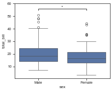

02 scatter

from kplot.scatter import reduce_feature, plot_2d, plot_cluster, plot_rel

import seaborn as sns

# Set up the objects used by the examples below.
df = sns.load_dataset('penguins').dropna().reset_index(drop=True)
df2 = df[['bill_length_mm', 'bill_depth_mm', 'flipper_length_mm', 'body_mass_g']]
print(df.shape)
print(df2.shape)

(333, 7)
(333, 4)

# Reduce a feature matrix to a lower-dimensional embedding dataframe.
reduce_feature(df2, method='pca', n=2)

	PCA1	PCA2
0	-457.325073	-13.351587
1	-407.252205	-9.179113
2	-957.044676	8.160444
3	-757.115802	1.867653
4	-557.177302	-3.389158
...	...	...
328	718.068699	2.338199
329	643.090909	4.280699
330	1543.098355	-2.232010
331	992.994900	-4.605154
332	1193.002584	-5.417312

333 rows × 2 columns

# Plot the first two columns of an embedding dataframe.
df2 = reduce_feature(df[['bill_length_mm', 'bill_depth_mm', 'flipper_length_mm', 'body_mass_g']], method='pca', n=2)
df2['species'] = df['species'].values
plot_2d(df2, hue='species', legend=True)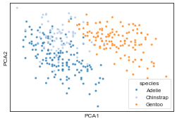

# Reduce features and immediately plot the first two embedding dimensions.
plot_cluster(df[['bill_length_mm', 'bill_depth_mm', 'flipper_length_mm', 'body_mass_g', 'species']], method='pca', hue='species', legend=True)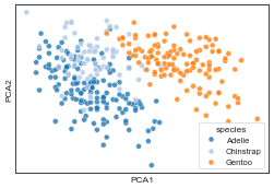

# Plot a pairwise relationship with an optional correlation annotation.
df2 = df[['bill_length_mm', 'flipper_length_mm', 'species']].head(12).copy()
df2.index = [f'pt{i}' for i in range(len(df2))]
plot_rel(df2, x='bill_length_mm', y='flipper_length_mm', hue='species', index_list=['pt0', 'pt11'])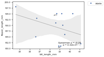

03 bar

from kplot.bar import plot_hist, plot_count, plot_bar, plot_group_bar, plot_stacked, plot_violin, plot_box, plot_pie, plot_cnt, calculate_pct, plot_composition

import seaborn as sns

# Set up the objects used by the examples below.
df = sns.load_dataset('tips').dropna()
df.shape

(244, 7)

# Plot a histogram with a KDE overlay and polygon bins.
plot_hist(df, 'total_bill')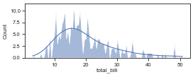

# Plot horizontal counts from a value-count series.
plot_count(df['day'].value_counts())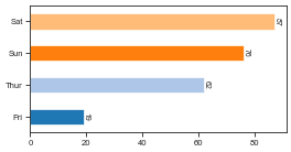

# Plot a bar chart from an unstacked dataframe.
plot_bar(df, value='total_bill', group='day')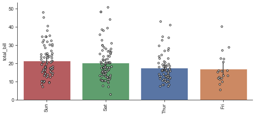

# Plot grouped bars after melting multiple value columns.
plot_group_bar(df, value_cols=['total_bill', 'tip'], group='day')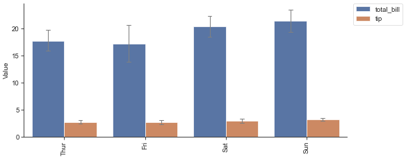

# Plot stacked counts for a categorical column.
plot_stacked(df, group='day', hue='sex')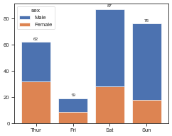

# Plot violin plots with optional strip dots.
df2 = df[['time', 'total_bill']].rename(columns={'time': 'variable', 'total_bill': 'value'})
plot_violin(df2)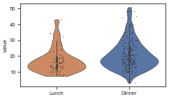

# Plot a box plot ordered by the group median.
plot_box(df, value='total_bill', group='day')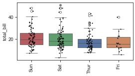

# Plot a pie chart from a value-count series.
plot_pie(df['day'].value_counts())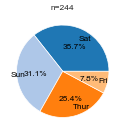

# Plot vertical counts with labels above the bars.
plot_cnt(df['day'].value_counts())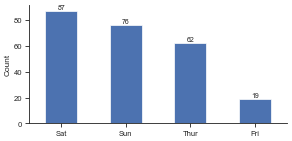

# Calculate within-bin percentages for a stacked composition chart.
df2 = sns.load_dataset('titanic').dropna(subset=['class', 'sex']).reset_index(drop=True)
calculate_pct(df2, 'class', 'sex')

sex	female	male
class
First	43.518519	56.481481
Second	41.304348	58.695652
Third	29.327902	70.672098

# Plot stacked percentages for a bin-by-category composition.
plot_composition(df2, 'class', 'sex')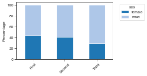

04 heatmap

from kplot.heatmap import get_similarity, plot_corr, plot_confusion_matrix

import seaborn as sns

# Set up the objects used by the examples below.
df = sns.load_dataset('titanic').dropna(subset=['age', 'fare', 'class', 'sex', 'survived']).reset_index(drop=True)
df2 = df[['age', 'fare', 'sibsp', 'parch']].head(8).copy()
df2.index = [f'row_{i}' for i in range(len(df2))]
print(df.shape)
print(df2.shape)

(714, 15)
(8, 4)

# Calculate both distance and similarity matrices for a dataframe.
get_similarity(df2)[0]

	row_0	row_1	row_2	row_3	row_4	row_5	row_6	row_7
row_0	0.000000	66.001996	4.177993	47.657345	13.062925	54.911521	24.415786	6.714166
row_1	66.001996	0.000000	64.492435	18.429118	63.312323	25.182682	61.821302	61.188418
row_2	4.177993	64.492435	0.000000	46.073643	9.000868	52.100901	27.548548	3.910651
row_3	47.657345	18.429118	46.073643	0.000000	45.061097	19.066500	46.039121	42.780883
row_4	13.062925	63.312323	9.000868	45.061097	0.000000	47.754949	35.618122	8.803791
row_5	54.911521	25.182682	52.100901	19.066500	47.754949	0.000000	60.513388	48.906725
row_6	24.415786	61.821302	27.548548	46.039121	35.618122	60.513388	0.000000	27.089433
row_7	6.714166	61.188418	3.910651	42.780883	8.803791	48.906725	27.089433	0.000000

# Plot a square matrix with an optional triangular mask.
plot_corr(df[['age', 'fare', 'sibsp', 'parch']].corr(numeric_only=True))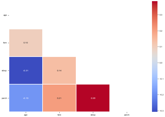

# Plot a confusion matrix from target and prediction arrays.
plot_confusion_matrix(df['survived'], df['adult_male'], class_names=['False', 'True'], normalize=True)

Normalized confusion matrix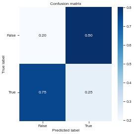

05 hierarchical

from kplot.hierarchical import get_1d_distance, get_1d_distance_parallel, get_Z, plot_dendrogram, get_hcluster

import pandas as pd,numpy as np,seaborn as sns
from scipy.spatial.distance import euclidean

# Set up the objects used by the examples below.
df0=sns.load_dataset("iris")
df = df0.drop(columns="species")

def my_distance(u, v):
    return np.sum(np.abs(u - v))

A = np.array([[0, 0], [1, 1], [2, 2]])

df0.head()

	sepal_length	sepal_width	petal_length	petal_width	species
0	5.1	3.5	1.4	0.2	setosa
1	4.9	3.0	1.4	0.2	setosa
2	4.7	3.2	1.3	0.2	setosa
3	4.6	3.1	1.5	0.2	setosa
4	5.0	3.6	1.4	0.2	setosa

# Compute 1D distance (like pdist from scipy) but for df with column names
# return 1d distance
get_1d_distance(pd.DataFrame(A),func_flat=my_distance)

100%|██████████| 3/3 [00:00<00:00, 3381.59it/s]

array([2, 4, 2])

# Parallel compute 1D distance for each row in a dataframe given a distance function
# get_1d_distance_parallel(df, func_flat=my_distance)

# Get linkage matrix Z from pssms dataframe
Z = get_Z(df,func_flat=euclidean,parallel=False)

100%|██████████| 150/150 [00:00<00:00, 532.10it/s]

# Run the example.
plot_dendrogram(Z,dense=10,labels=df.index,thr=0.5)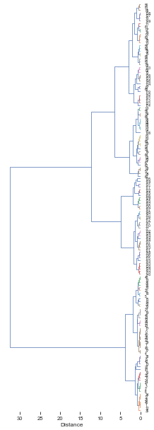

# Get flat cluster assignments from hierarchical clustering linkage matrix `Z`.
get_hcluster(df,labels=df0['species'].tolist(),thr=5,dense=10)

0      1
1      1
2      1
3      1
4      1
      ..
145    2
146    4
147    2
148    2
149    4
Length: 150, dtype: int32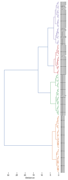

06 ranking

from kplot.ranking import plot_rank, get_AUCDF

import seaborn as sns

# Set up the objects used by the examples below.
df = sns.load_dataset('tips')
df.shape

(244, 7)

# Plot a ranked scatter and annotate the highest and lowest entries.
sort_df=df.sort_values('total_bill').copy()
sort_df['id'] = sort_df.index.astype(str)

plot_rank(sort_df, x='id', y='total_bill', n_hi=10, n_lo=10)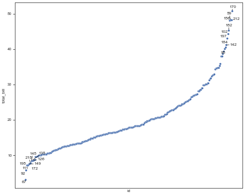

# Compute the normalized area under an empirical CDF over rank values.
get_AUCDF(df, 'total_bill', plot=True)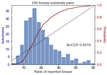

0.6519265042202643