df = sns.load_dataset('penguins').dropna().reset_index(drop=True)
df2 = df[['bill_length_mm', 'bill_depth_mm', 'flipper_length_mm', 'body_mass_g']]
print(df.shape)
print(df2.shape)
(333, 7)
(333, 4)df = sns.load_dataset('penguins').dropna().reset_index(drop=True)
df2 = df[['bill_length_mm', 'bill_depth_mm', 'flipper_length_mm', 'body_mass_g']]
print(df.shape)
print(df2.shape)(333, 7)
(333, 4)df.head()| species | island | bill_length_mm | bill_depth_mm | flipper_length_mm | body_mass_g | sex | |
|---|---|---|---|---|---|---|---|
| 0 | Adelie | Torgersen | 39.1 | 18.7 | 181.0 | 3750.0 | Male |
| 1 | Adelie | Torgersen | 39.5 | 17.4 | 186.0 | 3800.0 | Female |
| 2 | Adelie | Torgersen | 40.3 | 18.0 | 195.0 | 3250.0 | Female |
| 3 | Adelie | Torgersen | 36.7 | 19.3 | 193.0 | 3450.0 | Female |
| 4 | Adelie | Torgersen | 39.3 | 20.6 | 190.0 | 3650.0 | Male |
def reduce_feature(
    df:DataFrame, # numeric feature matrix
    method:str='pca', # one of pca, tsne, umap
    complexity:int=20, # perplexity for tsne or neighbors for umap
    n:int=2, # number of output dimensions
    load:str | pathlib.Path | None=None, # path to a previously fitted reducer
    save:str | pathlib.Path | None=None, # optional path for persisting the reducer
    seed:int=123, # random_state used by reducers that support it
    kwargs:VAR_KEYWORD
)->DataFrame: # forwarded reducer kwargs
Reduce a feature matrix to a lower-dimensional embedding dataframe.
reduce_feature(df2, method='pca', n=2)| PCA1 | PCA2 | |
|---|---|---|
| 0 | -457.325073 | -13.351587 |
| 1 | -407.252205 | -9.179113 |
| 2 | -957.044676 | 8.160444 |
| 3 | -757.115802 | 1.867653 |
| 4 | -557.177302 | -3.389158 |
| ... | ... | ... |
| 328 | 718.068699 | 2.338199 |
| 329 | 643.090909 | 4.280699 |
| 330 | 1543.098355 | -2.232010 |
| 331 | 992.994900 | -4.605154 |
| 332 | 1193.002584 | -5.417312 |
333 rows × 2 columns
def plot_2d(
    embedding_df:DataFrame, # dataframe with at least two numeric columns
    hue:str | None=None, # column name used for color when present in embedding_df
    palette:str='tab20', # seaborn palette name
    legend:bool=False, # whether to draw a legend
    name_list:list[str] | None=None, # labels used to annotate points
    s:int=20, # marker size
    legend_title:str | None=None, # optional legend title override
    kwargs:VAR_KEYWORD
):
Plot the first two columns of an embedding dataframe.
df2 = reduce_feature(df[['bill_length_mm', 'bill_depth_mm', 'flipper_length_mm', 'body_mass_g']], method='pca', n=2)
df2['species'] = df['species'].values
plot_2d(df2, hue='species', legend=True)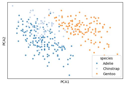
def plot_cluster(
    df:DataFrame, # numeric feature matrix, optionally including a hue column
    method:str='pca', # one of pca, tsne, umap
    hue:str | pandas.Series | list | None=None, # hue column name or per-row hue values
    complexity:int=30, # perplexity for tsne or neighbors for umap
    palette:str='tab20', # seaborn palette name
    legend:bool=False, # whether to draw a legend
    name_list:list[str] | None=None, # point annotations
    seed:int=123, # random seed passed to the reducer
    s:int=50, # marker size
    legend_title:str | None=None, # optional legend title override
    kwargs:VAR_KEYWORD
):
Reduce features and immediately plot the first two embedding dimensions.
plot_cluster(df[['bill_length_mm', 'bill_depth_mm', 'flipper_length_mm', 'body_mass_g', 'species']], method='pca', hue='species', legend=True)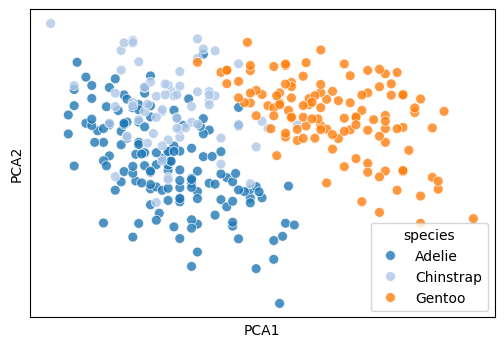
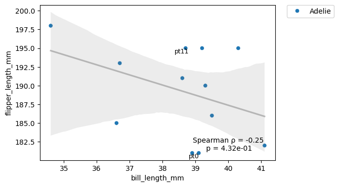
def plot_rel(
    df:DataFrame, # dataframe that contains the x and y columns
    x:str, # x-axis column name
    y:str, # y-axis column name
    text_location:tuple=(0.8, 0.1), # annotation location in axes coordinates
    method:str | None='spearman', # one of spearman, pearson, or None
    index_list:list[str] | None=None, # row labels to annotate
    hue:str | None=None, # optional categorical hue column
    reg_line:bool=True, # whether to draw a regression line when hue is used
    data:NoneType=None, x_estimator:NoneType=None, x_bins:NoneType=None, x_ci:str='ci', scatter:bool=True,
    fit_reg:bool=True, ci:int=95, n_boot:int=1000, units:NoneType=None, seed:NoneType=None, order:int=1,
    logistic:bool=False, lowess:bool=False, robust:bool=False, logx:bool=False, x_partial:NoneType=None,
    y_partial:NoneType=None, truncate:bool=True, dropna:bool=True, x_jitter:NoneType=None, y_jitter:NoneType=None,
    label:NoneType=None, color:NoneType=None, marker:str='o', scatter_kws:NoneType=None, line_kws:NoneType=None,
    ax:NoneType=None
):
Plot a pairwise relationship with an optional correlation annotation.
df2 = df[['bill_length_mm', 'flipper_length_mm', 'species']].head(12).copy()
df2.index = [f'pt{i}' for i in range(len(df2))]
plot_rel(df2, x='bill_length_mm', y='flipper_length_mm', hue='species', index_list=['pt0', 'pt11'])