bar

Categorical, count, distribution, and composition plot helpers.

df = sns.load_dataset('tips').dropna()
df.shape

(244, 7)

df.head()

	total_bill	tip	sex	smoker	day	time	size
0	16.99	1.01	Female	No	Sun	Dinner	2
1	10.34	1.66	Male	No	Sun	Dinner	3
2	21.01	3.50	Male	No	Sun	Dinner	3
3	23.68	3.31	Male	No	Sun	Dinner	2
4	24.59	3.61	Female	No	Sun	Dinner	4

Distribution Plots

---

plot_hist

def plot_hist(
    df:DataFrame, # dataframe containing the values to plot
    x:str, # numeric column name
    figsize:tuple=(6, 2), # figure size in inches
    data:NoneType=None, y:NoneType=None, hue:NoneType=None, weights:NoneType=None, # Vector variables
    stat:str='count', bins:str='auto', binwidth:NoneType=None,
    binrange:NoneType=None, # Histogram computation parameters
    discrete:NoneType=None, cumulative:bool=False, common_bins:bool=True, common_norm:bool=True,
    multiple:str='layer', element:str='bars', fill:bool=True, shrink:int=1, # Histogram appearance parameters
    kde:bool=False, kde_kws:NoneType=None,
    line_kws:NoneType=None, # Histogram smoothing with a kernel density estimate
    thresh:int=0, pthresh:NoneType=None, pmax:NoneType=None, cbar:bool=False, cbar_ax:NoneType=None,
    cbar_kws:NoneType=None, # Bivariate histogram parameters
    palette:NoneType=None, hue_order:NoneType=None, hue_norm:NoneType=None,
    color:NoneType=None, # Hue mapping parameters
    log_scale:NoneType=None, legend:bool=True, ax:NoneType=None, # Axes information
):

Plot a histogram with a KDE overlay and polygon bins.

plot_hist(df, 'total_bill')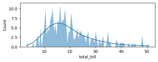

Count And Bar Plots

---

plot_count

def plot_count(
    cnt:Series, # output of df[col].value_counts()
    tick_spacing:float | None=None, # optional major tick interval
    palette:str='tab20', # seaborn palette name
):

Plot horizontal counts from a value-count series.

plot_count(df['day'].value_counts())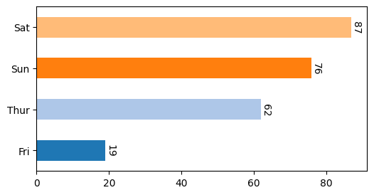

---

plot_bar

def plot_bar(
    df:DataFrame, # long-form dataframe
    value:str, # numeric column name
    group:str, # grouping column name
    title:str | None=None, # optional plot title
    figsize:tuple=(12, 5), # figure size in inches
    fontsize:int=14, # axis label and tick size
    dots:bool=True, # whether to overlay strip dots
    rotation:float=90, # x tick rotation angle
    ascending:bool=False, # sort group means ascending when True
    ymin:float | None=None, # optional lower y-axis bound
    data:NoneType=None, x:NoneType=None, y:NoneType=None, hue:NoneType=None, order:NoneType=None,
    hue_order:NoneType=None, estimator:str='mean', errorbar:tuple=('ci', 95), n_boot:int=1000, seed:NoneType=None,
    units:NoneType=None, weights:NoneType=None, orient:NoneType=None, color:NoneType=None, palette:NoneType=None,
    saturation:float=0.75, fill:bool=True, hue_norm:NoneType=None, width:float=0.8, dodge:str='auto', gap:int=0,
    log_scale:NoneType=None, native_scale:bool=False, formatter:NoneType=None, legend:str='auto', capsize:int=0,
    err_kws:NoneType=None, ci:Deprecated=<deprecated>, errcolor:Deprecated=<deprecated>,
    errwidth:Deprecated=<deprecated>, ax:NoneType=None
):

Plot a bar chart from an unstacked dataframe.

plot_bar(df, value='total_bill', group='day')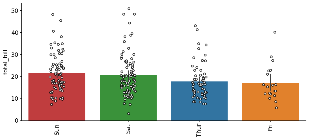

---

plot_group_bar

def plot_group_bar(
    df:DataFrame, # wide-form dataframe
    value_cols:list, # numeric columns to melt into grouped bars
    group:str, # grouping column preserved during melt
    figsize:tuple=(12, 5), # figure size in inches
    order:NoneType=None, # optional x order passed to seaborn
    title:str | None=None, # optional plot title
    fontsize:int=14, # axis label and tick size
    rotation:float=90, # x tick rotation angle
    data:NoneType=None, x:NoneType=None, y:NoneType=None, hue:NoneType=None, hue_order:NoneType=None,
    estimator:str='mean', errorbar:tuple=('ci', 95), n_boot:int=1000, seed:NoneType=None, units:NoneType=None,
    weights:NoneType=None, orient:NoneType=None, color:NoneType=None, palette:NoneType=None, saturation:float=0.75,
    fill:bool=True, hue_norm:NoneType=None, width:float=0.8, dodge:str='auto', gap:int=0, log_scale:NoneType=None,
    native_scale:bool=False, formatter:NoneType=None, legend:str='auto', capsize:int=0, err_kws:NoneType=None,
    ci:Deprecated=<deprecated>, errcolor:Deprecated=<deprecated>, errwidth:Deprecated=<deprecated>, ax:NoneType=None
):

Plot grouped bars after melting multiple value columns.

plot_group_bar(df, value_cols=['total_bill', 'tip'], group='day')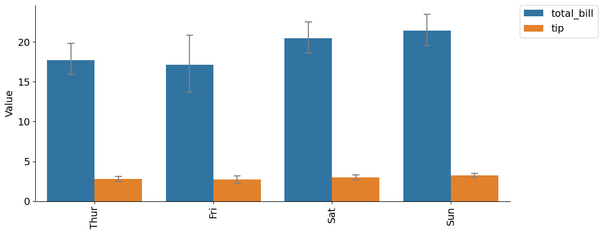

---

plot_stacked

def plot_stacked(
    df:DataFrame, # dataframe containing the stacked categories
    group:str, # x-axis categorical column
    hue:str, # stacked hue column
    figsize:tuple=(5, 4), # figure size in inches
    xlabel:str | None=None, # x-axis label override
    ylabel:str | None=None, # y-axis label override
    add_value:bool=True, # whether to annotate total counts
    kwargs:VAR_KEYWORD
):

Plot stacked counts for a categorical column.

plot_stacked(df, group='day', hue='sex')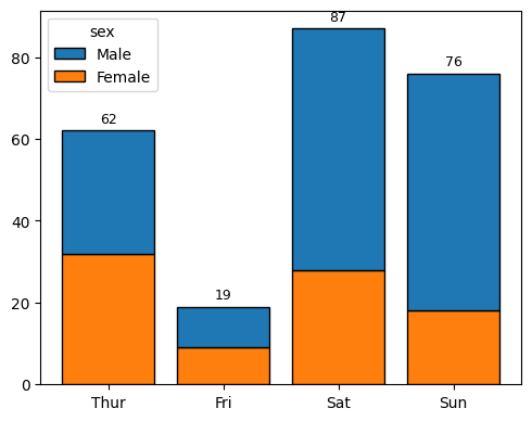

Distribution Comparisons

---

plot_violin

def plot_violin(
    df:DataFrame, # long-form dataframe with value and group columns
    value:str='value', # numeric column name
    group:str='variable', # grouping column name
    ylabel:str | None=None, # optional y-axis label override
    dots:bool=True, # whether to overlay strip dots
    figsize:tuple=(5, 3), # figure size in inches
    kwargs:VAR_KEYWORD
):

Plot violin plots with optional strip dots.

df2 = df[['time', 'total_bill']].rename(columns={'time': 'variable', 'total_bill': 'value'})
plot_violin(df2)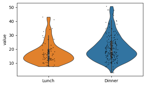

---

plot_box

def plot_box(
    df:DataFrame, # long-form dataframe
    value:str, # numeric column name
    group:str, # grouping column name
    title:str | None=None, # optional plot title
    figsize:tuple=(6, 3), # figure size in inches
    fontsize:int=14, # axis label and tick size
    dots:bool=True, # whether to overlay strip dots
    rotation:float=90, # x tick rotation angle
    data:NoneType=None, x:NoneType=None, y:NoneType=None, hue:NoneType=None, order:NoneType=None,
    hue_order:NoneType=None, orient:NoneType=None, color:NoneType=None, palette:NoneType=None, saturation:float=0.75,
    fill:bool=True, dodge:str='auto', width:float=0.8, gap:int=0, whis:float=1.5, linecolor:str='auto',
    linewidth:NoneType=None, fliersize:NoneType=None, hue_norm:NoneType=None, native_scale:bool=False,
    log_scale:NoneType=None, formatter:NoneType=None, legend:str='auto', ax:NoneType=None
):

Plot a box plot ordered by the group median.

plot_box(df, value='total_bill', group='day')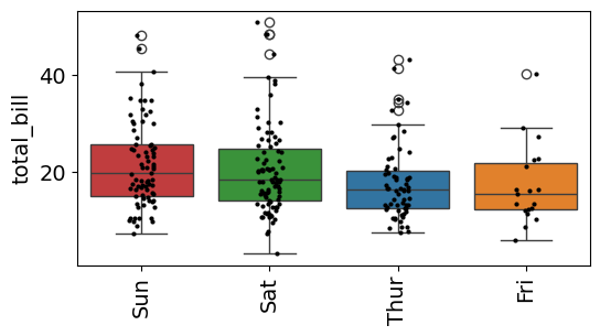

Pie And Count Labels

---

plot_pie

def plot_pie(
    value_counts:Series, # categorical counts
    hue_order:list[str] | None=None, # explicit slice order
    labeldistance:float=0.8, # distance of labels from the center
    fontsize:int=12, # label font size
    font_color:str='black', # label font color
    palette:str='tab20', # seaborn palette name
    figsize:tuple=(4, 3), # figure size in inches
):

Plot a pie chart from a value-count series.

plot_pie(df['day'].value_counts())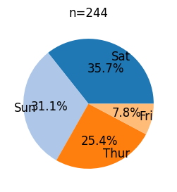

---

plot_cnt

def plot_cnt(
    cnt:Series, # output of df[col].value_counts()
    xlabel:str | None=None, # x-axis label override
    ylabel:str='Count', # y-axis label override
    figsize:tuple=(6, 3), # figure size in inches
):

Plot vertical counts with labels above the bars.

plot_cnt(df['day'].value_counts())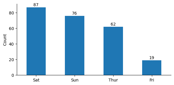

Composition

---

calculate_pct

def calculate_pct(
    df:DataFrame, # source dataframe
    bin_col:str, # binned x-axis column
    hue_col:str, # stacked hue column
)->DataFrame:

Calculate within-bin percentages for a stacked composition chart.

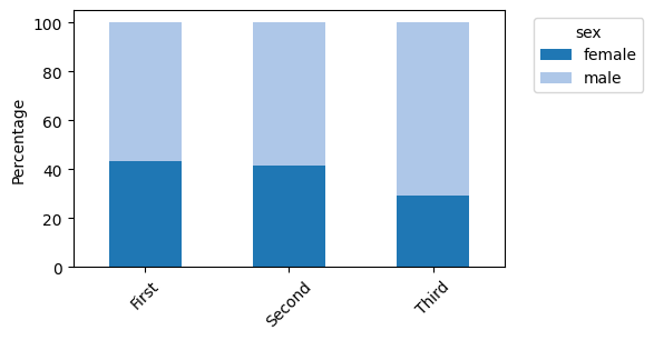
df2 = sns.load_dataset('titanic').dropna(subset=['class', 'sex']).reset_index(drop=True)
calculate_pct(df2, 'class', 'sex')

sex	female	male
class
First	43.518519	56.481481
Second	41.304348	58.695652
Third	29.327902	70.672098

---

plot_composition

def plot_composition(
    df:DataFrame, # source dataframe
    bin_col:str, # binned x-axis column
    hue_col:str, # stacked hue column
    palette:dict | list | str='tab20', # colors passed to get_plt_color
    legend_title:str | None=None, # legend title override
    rotation:float=45, # x tick rotation angle
    xlabel:str | None=None, # x-axis label override
    ylabel:str='Percentage', # y-axis label override
    figsize:tuple=(5, 3), # figure size in inches
):

Plot stacked percentages for a bin-by-category composition.

plot_composition(df2, 'class', 'sex')